写给程序员的机器学习入门 (九) - 对象识别 RCNN 与 Fast-RCNN （二）

使用 RCNN 学习与识别这些图片中的人脸区域的代码如下：

import os
import sys
import torch
import gzip
import itertools
import random
import numpy
import pandas
import torchvision
import cv2
from torch import nn
from matplotlib import pyplot
from collections import defaultdict

# 各个区域缩放到的图片大小
REGION_IMAGE_SIZE = (32, 32)
# 分析目标的图片所在的文件夹
IMAGE_DIR = "./784145_1347673_bundle_archive/train/image_data"
# 定义各个图片中人脸区域的 CSV 文件
BOX_CSV_PATH = "./784145_1347673_bundle_archive/train/bbox_train.csv"

# 用于启用 GPU 支持
device = torch.device("cuda" if torch.cuda.is_available() else "cpu")

class MyModel(nn.Module):
    """识别是否人脸 (ResNet-18)"""
    def __init__(self):
        super().__init__()
        # Resnet 的实现
        # 输出两个分类 [非人脸, 人脸]
        self.resnet = torchvision.models.resnet18(num_classes=2)

    def forward(self, x):
        # 应用 ResNet
        y = self.resnet(x)
        return y

def save_tensor(tensor, path):
    """保存 tensor 对象到文件"""
    torch.save(tensor, gzip.GzipFile(path, "wb"))

def load_tensor(path):
    """从文件读取 tensor 对象"""
    return torch.load(gzip.GzipFile(path, "rb"))

def image_to_tensor(img):
    """转换 opencv 图片对象到 tensor 对象"""
    # 注意 opencv 是 BGR，但对训练没有影响所以不用转为 RGB
    img = cv2.resize(img, dsize=REGION_IMAGE_SIZE)
    arr = numpy.asarray(img)
    t = torch.from_numpy(arr)
    t = t.transpose(0, 2) # 转换维度 H,W,C 到 C,W,H
    t = t / 255.0 # 正规化数值使得范围在 0 ~ 1
    return t

def calc_iou(rect1, rect2):
    """计算两个区域重叠部分 / 合并部分的比率 (intersection over union)"""
    x1, y1, w1, h1 = rect1
    x2, y2, w2, h2 = rect2
    xi = max(x1, x2)
    yi = max(y1, y2)
    wi = min(x1+w1, x2+w2) - xi
    hi = min(y1+h1, y2+h2) - yi
    if wi > 0 and hi > 0: # 有重叠部分
        area_overlap = wi*hi
        area_all = w1*h1 + w2*h2 - area_overlap
        iou = area_overlap / area_all
    else: # 没有重叠部分
        iou = 0
    return iou

def selective_search(img):
    """计算 opencv 图片中可能出现对象的区域，只返回头 2000 个区域"""
    # 算法参考 https://www.learnopencv.com/selective-search-for-object-detection-cpp-python/
    s = cv2.ximgproc.segmentation.createSelectiveSearchSegmentation()
    s.setBaseImage(img)
    s.switchToSelectiveSearchFast()
    boxes = s.process()
    return boxes[:2000]

def prepare_save_batch(batch, image_tensors, image_labels):
    """准备训练 - 保存单个批次的数据"""
    # 生成输入和输出 tensor 对象
    tensor_in = torch.stack(image_tensors) # 维度: B,C,W,H
    tensor_out = torch.tensor(image_labels, dtype=torch.long) # 维度: B

    # 切分训练集 (80%)，验证集 (10%) 和测试集 (10%)
    random_indices = torch.randperm(tensor_in.shape[0])
    training_indices = random_indices[:int(len(random_indices)*0.8)]
    validating_indices = random_indices[int(len(random_indices)*0.8):int(len(random_indices)*0.9):]
    testing_indices = random_indices[int(len(random_indices)*0.9):]
    training_set = (tensor_in[training_indices], tensor_out[training_indices])
    validating_set = (tensor_in[validating_indices], tensor_out[validating_indices])
    testing_set = (tensor_in[testing_indices], tensor_out[testing_indices])

    # 保存到硬盘
    save_tensor(training_set, f"data/training_set.{batch}.pt")
    save_tensor(validating_set, f"data/validating_set.{batch}.pt")
    save_tensor(testing_set, f"data/testing_set.{batch}.pt")
    print(f"batch {batch} saved")

def prepare():
    """准备训练"""
    # 数据集转换到 tensor 以后会保存在 data 文件夹下
    if not os.path.isdir("data"):
        os.makedirs("data")

    # 加载 csv 文件，构建图片到区域列表的索引 { 图片名: [ 区域, 区域, .. ] }
    box_map = defaultdict(lambda: [])
    df = pandas.read_csv(BOX_CSV_PATH)
    for row in df.values:
        filename, width, height, x1, y1, x2, y2 = row[:7]
        box_map[filename].append((x1, y1, x2-x1, y2-y1))

    # 从图片里面提取人脸 (正样本) 和非人脸 (负样本) 的图片
    batch_size = 1000
    batch = 0
    image_tensors = []
    image_labels = []
    for filename, true_boxes in box_map.items():
        path = os.path.join(IMAGE_DIR, filename)
        img = cv2.imread(path) # 加载原始图片
        candidate_boxes = selective_search(img) # 查找候选区域
        positive_samples = 0
        negative_samples = 0
        for candidate_box in candidate_boxes:
            # 如果候选区域和任意一个实际区域重叠率大于 70%，则认为是正样本
            # 如果候选区域和所有实际区域重叠率都小于 30%，则认为是负样本
            # 每个图片最多添加正样本数量 + 10 个负样本，需要提供足够多负样本避免伪阳性判断
            iou_list = [ calc_iou(candidate_box, true_box) for true_box in true_boxes ]
            positive_index = next((index for index, iou in enumerate(iou_list) if iou > 0.70), None)
            is_negative = all(iou < 0.30 for iou in iou_list)
            result = None
            if positive_index is not None:
                result = True
                positive_samples += 1
            elif is_negative and negative_samples < positive_samples + 10:
                result = False
                negative_samples += 1
            if result is not None:
                x, y, w, h = candidate_box
                child_img = img[y:y+h, x:x+w].copy()
                # 检验计算是否有问题
                # cv2.imwrite(f"{filename}_{x}_{y}_{w}_{h}_{int(result)}.png", child_img)
                image_tensors.append(image_to_tensor(child_img))
                image_labels.append(int(result))
                if len(image_tensors) >= batch_size:
                    # 保存批次
                    prepare_save_batch(batch, image_tensors, image_labels)
                    image_tensors.clear()
                    image_labels.clear()
                    batch += 1
    # 保存剩余的批次
    if len(image_tensors) > 10:
        prepare_save_batch(batch, image_tensors, image_labels)

def train():
    """开始训练"""
    # 创建模型实例
    model = MyModel().to(device)

    # 创建损失计算器
    loss_function = torch.nn.CrossEntropyLoss()

    # 创建参数调整器
    optimizer = torch.optim.Adam(model.parameters())

    # 记录训练集和验证集的正确率变化
    training_accuracy_history = []
    validating_accuracy_history = []

    # 记录最高的验证集正确率
    validating_accuracy_highest = -1
    validating_accuracy_highest_epoch = 0

    # 读取批次的工具函数
    def read_batches(base_path):
        for batch in itertools.count():
            path = f"{base_path}.{batch}.pt"
            if not os.path.isfile(path):
                break
            yield [ t.to(device) for t in load_tensor(path) ]

    # 计算正确率的工具函数，正样本和负样本的正确率分别计算再平均
    def calc_accuracy(actual, predicted):
        predicted = torch.max(predicted, 1).indices
        acc_positive = ((actual > 0.5) & (predicted > 0.5)).sum().item() / ((actual > 0.5).sum().item() + 0.00001)
        acc_negative = ((actual <= 0.5) & (predicted <= 0.5)).sum().item() / ((actual <= 0.5).sum().item() + 0.00001)
        acc = (acc_positive + acc_negative) / 2
        return acc
 
    # 划分输入和输出的工具函数
    def split_batch_xy(batch, begin=None, end=None):
        # shape = batch_size, channels, width, height
        batch_x = batch[0][begin:end]
        # shape = batch_size, num_labels
        batch_y = batch[1][begin:end]
        return batch_x, batch_y

    # 开始训练过程
    for epoch in range(1, 10000):
        print(f"epoch: {epoch}")

        # 根据训练集训练并修改参数
        model.train()
        training_accuracy_list = []
        for batch_index, batch in enumerate(read_batches("data/training_set")):
            # 切分小批次，有助于泛化模型
            training_batch_accuracy_list = []
            for index in range(0, batch[0].shape[0], 100):
                # 划分输入和输出
                batch_x, batch_y = split_batch_xy(batch, index, index+100)
                # 计算预测值
                predicted = model(batch_x)
                # 计算损失
                loss = loss_function(predicted, batch_y)
                # 从损失自动微分求导函数值
                loss.backward()
                # 使用参数调整器调整参数
                optimizer.step()
                # 清空导函数值
                optimizer.zero_grad()
                # 记录这一个批次的正确率，torch.no_grad 代表临时禁用自动微分功能
                with torch.no_grad():
                    training_batch_accuracy_list.append(calc_accuracy(batch_y, predicted))
            # 输出批次正确率
            training_batch_accuracy = sum(training_batch_accuracy_list) / len(training_batch_accuracy_list)
            training_accuracy_list.append(training_batch_accuracy)
            print(f"epoch: {epoch}, batch: {batch_index}: batch accuracy: {training_batch_accuracy}")
        training_accuracy = sum(training_accuracy_list) / len(training_accuracy_list)
        training_accuracy_history.append(training_accuracy)
        print(f"training accuracy: {training_accuracy}")

        # 检查验证集
        model.eval()
        validating_accuracy_list = []
        for batch in read_batches("data/validating_set"):
            batch_x, batch_y = split_batch_xy(batch)
            predicted = model(batch_x)
            validating_accuracy_list.append(calc_accuracy(batch_y, predicted))
        validating_accuracy = sum(validating_accuracy_list) / len(validating_accuracy_list)
        validating_accuracy_history.append(validating_accuracy)
        print(f"validating accuracy: {validating_accuracy}")

        # 记录最高的验证集正确率与当时的模型状态，判断是否在 20 次训练后仍然没有刷新记录
        if validating_accuracy > validating_accuracy_highest:
            validating_accuracy_highest = validating_accuracy
            validating_accuracy_highest_epoch = epoch
            save_tensor(model.state_dict(), "model.pt")
            print("highest validating accuracy updated")
        elif epoch - validating_accuracy_highest_epoch > 20:
            # 在 20 次训练后仍然没有刷新记录，结束训练
            print("stop training because highest validating accuracy not updated in 20 epoches")
            break

    # 使用达到最高正确率时的模型状态
    print(f"highest validating accuracy: {validating_accuracy_highest}",
        f"from epoch {validating_accuracy_highest_epoch}")
    model.load_state_dict(load_tensor("model.pt"))

    # 检查测试集
    testing_accuracy_list = []
    for batch in read_batches("data/testing_set"):
        batch_x, batch_y = split_batch_xy(batch)
        predicted = model(batch_x)
        testing_accuracy_list.append(calc_accuracy(batch_y, predicted))
    testing_accuracy = sum(testing_accuracy_list) / len(testing_accuracy_list)
    print(f"testing accuracy: {testing_accuracy}")

    # 显示训练集和验证集的正确率变化
    pyplot.plot(training_accuracy_history, label="training")
    pyplot.plot(validating_accuracy_history, label="validing")
    pyplot.ylim(0, 1)
    pyplot.legend()
    pyplot.show()

def eval_model():
    """使用训练好的模型"""
    # 创建模型实例，加载训练好的状态，然后切换到验证模式
    model = MyModel().to(device)
    model.load_state_dict(load_tensor("model.pt"))
    model.eval()

    # 询问图片路径，并显示所有可能是人脸的区域
    while True:
        try:
            # 选取可能出现对象的区域一览
            image_path = input("Image path: ")
            if not image_path:
                continue
            img = cv2.imread(image_path)
            candidate_boxes = selective_search(img)
            # 构建输入
            image_tensors = []
            for candidate_box in candidate_boxes:
                x, y, w, h = candidate_box
                child_img = img[y:y+h, x:x+w].copy()
                image_tensors.append(image_to_tensor(child_img))
            tensor_in = torch.stack(image_tensors).to(device)
            # 预测输出
            tensor_out = model(tensor_in)
            # 使用 softmax 计算是人脸的概率
            tensor_out = nn.functional.softmax(tensor_out, dim=1)
            tensor_out = tensor_out[:,1].resize(tensor_out.shape[0])
            # 判断概率大于 99% 的是人脸，添加边框到图片并保存
            img_output = img.copy()
            indices = torch.where(tensor_out > 0.99)[0]
            result_boxes = []
            result_boxes_all = []
            for index in indices:
                box = candidate_boxes[index]
                for exists_box in result_boxes_all:
                    # 如果和现存找到的区域重叠度大于 30% 则跳过
                    if calc_iou(exists_box, box) > 0.30:
                        break
                else:
                    result_boxes.append(box)
                result_boxes_all.append(box)
            for box in result_boxes:
                x, y, w, h = box
                print(x, y, w, h)
                cv2.rectangle(img_output, (x, y), (x+w, y+h), (0, 0, 0xff), 1)
            cv2.imwrite("img_output.png", img_output)
            print("saved to img_output.png")
            print()
        except Exception as e:
            print("error:", e)

def main():
    """主函数"""
    if len(sys.argv) < 2:
        print(f"Please run: {sys.argv[0]} prepare|train|eval")
        exit()

    # 给随机数生成器分配一个初始值，使得每次运行都可以生成相同的随机数
    # 这是为了让过程可重现，你也可以选择不这样做
    random.seed(0)
    torch.random.manual_seed(0)

    # 根据命令行参数选择操作
    operation = sys.argv[1]
    if operation == "prepare":
        prepare()
    elif operation == "train":
        train()
    elif operation == "eval":
        eval_model()
    else:
        raise ValueError(f"Unsupported operation: {operation}")

if __name__ == "__main__":
    main()

和之前文章给出的代码例子一样，这份代码也分为了 prepare, train, eval 三个部分，其中 prepare 部分负责选取区域，提取正样本 (包含人脸的区域) 和负样本 (不包含人脸的区域) 的子图片；train 使用普通的 resnet 模型学习子图片；eval 针对给出的图片选取区域并识别所有区域中是否包含人脸。

除了选取区域和提取子图片的处理以外，基本上和之前介绍的 CNN 模型一样吧🥳。

执行以下命令以后：

python3 example.py prepare
python3 example.py train

的最终输出如下：

epoch: 101, batch: 106: batch accuracy: 0.9999996838862198
epoch: 101, batch: 107: batch accuracy: 0.999218446914751
epoch: 101, batch: 108: batch accuracy: 0.9999996211125055
training accuracy: 0.999441394076678
validating accuracy: 0.9687856357743619
stop training because highest validating accuracy not updated in 20 epoches
highest validating accuracy: 0.9766918253771755 from epoch 80
testing accuracy: 0.9729761086851993

训练集和验证集的正确率变化如下：

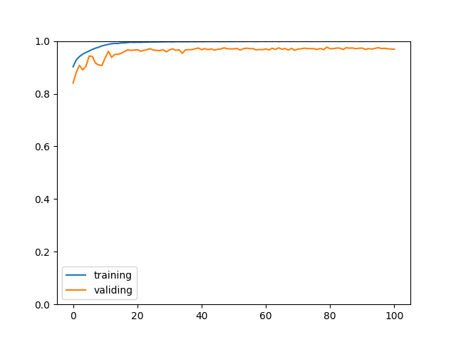
正确率看起来很高，但这只是针对选取后的区域判断的正确率，因为选取算法效果比较一般并且样本数量比较少，所以最终效果不能说令人满意😕。

执行以下命令，再输入图片路径可以使用学习好的模型识别图片：

python3 example.py eval

以下是部分识别结果：

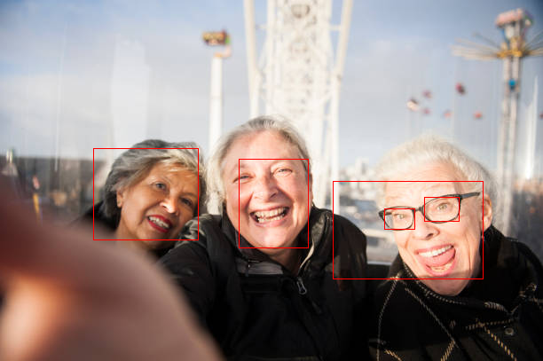
精度一般般😕。

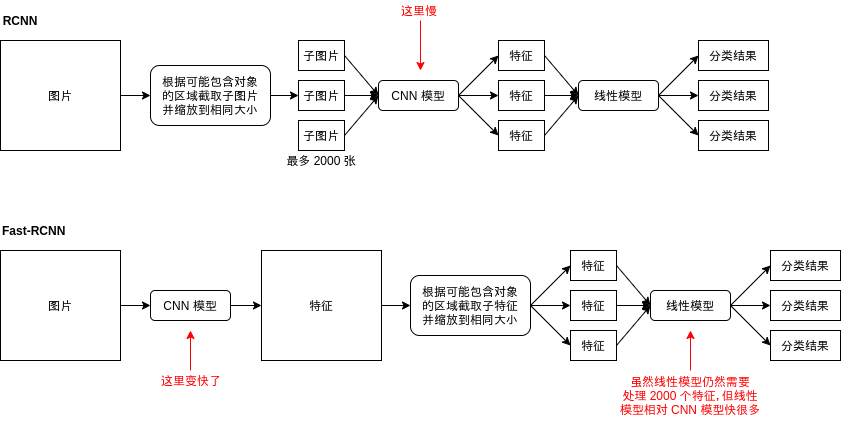
Fast-RCNN

RCNN 慢的原因主要是因为识别几千个子图片的计算量非常庞大，特别是这几千个子图片的范围很多是重合的，导致了很多重复的计算。Fast-RCNN 着重改善了这一部分，首先会针对整张图片生成一个与图片长宽相同 (或者等比例缩放) 的特征数据，然后再根据可能包含对象的区域截取特征数据，然后再根据截取后的子特征数据识别分类。RCNN 与 Fast-RCNN 的区别如下图所示：

遗憾的是 Fast-RCNN 只是改善了速度，并不会改善正确率。但下面介绍的例子会引入一个比较重要的处理，即调整区域范围，它可以让模型给出的区域更接近实际的区域。

以下是 Fast-RCNN 模型中的一些处理细节。

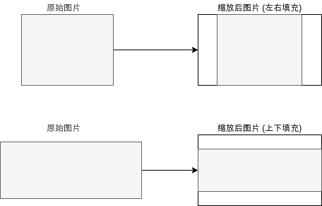
缩放来源图片

在 RCNN 中，传给 CNN 模型的图片是经过缩放的子图片，而在 Fast-RCNN 中我们需要传原图片给 CNN 模型，那么原图片也需要进行缩放。缩放使用的方法是填充法，如下图所示：

缩放图片使用的代码如下 (opencv 版)：

IMAGE_SIZE = (128, 88)

def calc_resize_parameters(sw, sh):
    """计算缩放图片的参数"""
    sw_new, sh_new = sw, sh
    dw, dh = IMAGE_SIZE
    pad_w, pad_h = 0, 0
    if sw / sh < dw / dh:
        sw_new = int(dw / dh * sh)
        pad_w = (sw_new - sw) // 2 # 填充左右
    else:
        sh_new = int(dh / dw * sw)
        pad_h = (sh_new - sh) // 2 # 填充上下
    return sw_new, sh_new, pad_w, pad_h

def resize_image(img):
    """缩放 opencv 图片，比例不一致时填充"""
    sh, sw, _ = img.shape
    sw_new, sh_new, pad_w, pad_h = calc_resize_parameters(sw, sh)
    img = cv2.copyMakeBorder(img, pad_h, pad_h, pad_w, pad_w, cv2.BORDER_CONSTANT, (0, 0, 0))
    img = cv2.resize(img, dsize=IMAGE_SIZE)
    return img

缩放图片后区域的坐标也需要转换，转换的代码如下 (都是枯燥的代码🤒)：

IMAGE_SIZE = (128, 88)

def map_box_to_resized_image(box, sw, sh):
    """把原始区域转换到缩放后的图片对应的区域"""
    x, y, w, h = box
    sw_new, sh_new, pad_w, pad_h = calc_resize_parameters(sw, sh)
    scale = IMAGE_SIZE[0] / sw_new
    x = int((x + pad_w) * scale)
    y = int((y + pad_h) * scale)
    w = int(w * scale)
    h = int(h * scale)
    if x + w > IMAGE_SIZE[0] or y + h > IMAGE_SIZE[1] or w == 0 or h == 0:
        return 0, 0, 0, 0
    return x, y, w, h

def map_box_to_original_image(box, sw, sh):
    """把缩放后图片对应的区域转换到缩放前的原始区域"""
    x, y, w, h = box
    sw_new, sh_new, pad_w, pad_h = calc_resize_parameters(sw, sh)
    scale = IMAGE_SIZE[0] / sw_new
    x = int(x / scale - pad_w)
    y = int(y / scale - pad_h)
    w = int(w / scale)
    h = int(h / scale)
    if x + w > sw or y + h > sh or x < 0 or y < 0 or w == 0 or h == 0:
        return 0, 0, 0, 0
    return x, y, w, h

计算区域特征

在前面的文章中我们已经了解过，CNN 模型可以分为卷积层，池化层和全连接层，卷积层，池化层用于抽取图片中各个区域的特征，全连接层用于把特征扁平化并交给线性模型处理。在 Fast-RCNN 中，我们不需要使用整张图片的特征，只需要使用部分区域的特征，所以 Fast-RCNN 使用的 CNN 模型只需要卷积层和池化层 (部分模型池化层可以省略)，卷积层输出的通道数量通常会比图片原有的通道数量多，并且长宽会按原来图片的长宽等比例缩小，例如原图的大小是 3,256,256 的时候，经过处理可能会输出 512,32,32，代表每个 8x8 像素的区域都对应 512 个特征。

这篇给出的 Fast-RCN 代码为了易于理解，会让 CNN 模型输出和原图一模一样的大小，这样抽取区域特征的时候只需要使用 [] 操作符即可。

抽取区域特征 (ROI Pooling)

Fast-RCNN 根据整张图片生成特征以后，下一步就是抽取区域特征 (Region of interest Pooling) 了，抽取区域特征简单的来说就是根据区域在图片中的位置，截区域中该位置的数据，然后再缩放到相同大小，如下图所示：

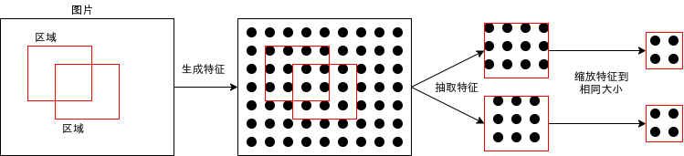
抽取区域特征的层又称为 ROI 层。

如果特征的长宽和图片的长宽相同，那么截取特征只需要简单的 [] 操作，但如果特征的长宽比图片的长宽要小，那么就需要使用近邻插值法 (Nearest Neighbor Interpolation) 或者双线插值法 (Bilinear Interpolation) 进行截取，使用双线插值法进行截取的 ROI 层又称作 ROI Align。截取以后的缩放可以使用 MaxPool，近邻插值法或双线插值法等算法。

想更好的理解 ROI Align 与双线插值法可以参考这篇文章。

调整区域范围

在前面已经提到过，使用选择搜索法等算法选取出来的区域与对象实际所在的区域可能有一定偏差，这个偏差是可以通过模型来调整的。举个简单的例子，如果区域内有脸的左半部分，那么模型在经过学习后应该可以判断出区域应该向右扩展一些。

区域调整可以分为四个参数：

• 对左上角 x 坐标的调整
• 对左上角 y 坐标的调整
• 对长度的调整
• 对宽度的调整

因为坐标和长宽的值大小不一定，例如同样是脸的左半部分，出现在图片的左上角和图片的右下角就会让 x y 坐标不一样，如果远近不同那么长宽也会不一样，我们需要把调整量作标准化，标准化的公式如下：

• x1, y1, w1, h1 = 候选区域
• x2, y2, w2, h2 = 真实区域
• x 偏移 = (x2 - x1) / w1
• y 偏移 = (y2 - y1) / h1
• w 偏移 = log(w2 / w1)
• h 偏移 = log(h2 / h1)

经过标准化后，偏移的值就会作为比例而不是绝对值，不会受具体坐标和长宽的影响。此外，公式中使用 log 是为了减少偏移的增幅，使得偏移比较大的时候模型仍然可以达到比较好的学习效果。

计算区域调整偏移和根据偏移调整区域的代码如下：

def calc_box_offset(candidate_box, true_box):
    """计算候选区域与实际区域的偏移值"""
    x1, y1, w1, h1 = candidate_box
    x2, y2, w2, h2 = true_box
    x_offset = (x2 - x1) / w1
    y_offset = (y2 - y1) / h1
    w_offset = math.log(w2 / w1)
    h_offset = math.log(h2 / h1)
    return (x_offset, y_offset, w_offset, h_offset)

def adjust_box_by_offset(candidate_box, offset):
    """根据偏移值调整候选区域"""
    x1, y1, w1, h1 = candidate_box
    x_offset, y_offset, w_offset, h_offset = offset
    x2 = w1 * x_offset + x1
    y2 = h1 * y_offset + y1
    w2 = math.exp(w_offset) * w1
    h2 = math.exp(h_offset) * h1
    return (x2, y2, w2, h2)