This paper presents the key algorithmic techniques behind CatBoost, a new gradient  boosting toolkit. Their combination leads to CatBoost outperforming other publicly  available boosting implementations in terms of quality on a variety of datasets.  Two critical algorithmic advances introduced in CatBoost are the implementation  of ordered boosting, a permutation-driven alternative to the classic algorithm, and  an innovative algorithm for processing categorical features. Both techniques were  created to fight a prediction shift caused by a special kind of target leakage present  in all currently existing implementations of gradient boosting algorithms. In this  paper, we provide a detailed analysis of this problem and demonstrate that proposed  algorithms solve it effectively, leading to excellent empirical results.

本文介绍了CatBoost（一种新的梯度增强工具包）背后的关键算法技术。它们的结合使得CatBoost在各种数据集上的质量优于其他公开可用的提升实施。CatBoost中引入的两个关键算法改进是有序增强(ordered boosting)的实现，这是一种排列驱动的替代经典算法，以及一种处理类别特征的创新算法。这两种技术都是为了应对当前所有梯度增强算法实现中存在的一种特殊类型的目标泄漏所造成的预测偏移。在本文中，我们对这一问题进行了详细的分析，并证明所提出的算法有效地解决了这一问题，并取得了良好的实证结果。

Gradient boosting is a powerful machine-learning technique that achieves state-of-the-art results in a  variety of practical tasks. For many years, it has remained the primary method for learning problems  with heterogeneous features, noisy data, and complex dependencies: web search, recommendation  systems, weather forecasting, and many others [5, 26, 29, 32]. Gradient boosting is essentially a  process of constructing an ensemble predictor by performing gradient descent in a functional space.  It is backed by solid theoretical results that explain how strong predictors can be built by iteratively  combining weaker models (base predictors) in a greedy manner [17].  

We show in this paper that all existing implementations of gradient boosting face the following  statistical issue. A prediction model F obtained after several steps of boosting relies on the targets  of all training examples. We demonstrate that this actually leads to a shift of the distribution of  F(xk) | xk for a training example xk from the distribution of F(x) | x for a test example x. This  finally leads to a prediction shift of the learned model. We identify this problem as a special kind of  target leakage in Section 4. Further, there is a similar issue in standard algorithms of preprocessing  categorical features. One of the most effective ways [6, 25] to use them in gradient boosting is  converting categories to their target statistics. A target statistic is a simple statistical model itself, and  it can also cause target leakage and a prediction shift. We analyze this in Section 3.  

梯度增强是一种功能强大的机器学习技术，可以在各种实际任务中获得最先进的结果。多年来，它一直是学习具有异质特征、噪声数据和复杂依赖关系问题的主要方法：网络web搜索、推荐系统、天气预报等[5,26,29,32]。梯度提升本质上是一个通过在函数空间中执行梯度下降来构造集合预测器的过程。它得到了可靠的理论结果的支持，解释了如何通过以贪婪的方式迭代地组合较弱的模型(基础预测器)来构建强大的预测器。

我们在这篇文章中表明，所有现有的梯度提升的实现面临以下统计问题。经过几步增强得到的预测模型F依赖于所有训练示例的目标。我们证明，这实际上导致训练示例xk的F(xk) | xk的分布从测试示例x的F(x) | x的分布转移。这最终导致学习模型的预测转移。在第四节中，我们将此问题定义为一种特殊的目标泄漏。此外，在分类特征预处理的标准算法中也存在类似的问题。在梯度提升中使用它们的最有效方法之一[6,25]是将类别转换为它们的目标统计信息。目标统计本身是一个简单的统计模型，它也可能导致目标泄漏和预测偏移。我们将在第3部分对此进行分析。

In this paper, we propose ordering principle to solve both problems. Relying on it, we derive  ordered boosting, a modification of standard gradient boosting algorithm, which avoids target  leakage (Section 4), and a new algorithm for processing categorical features (Section 3). Their  combination is implemented as an open-source library1  called CatBoost (for “Categorical Boosting”),  which outperforms the existing state-of-the-art implementations of gradient boosted decision trees —  XGBoost [8] and LightGBM [16] — on a diverse set of popular machine learning tasks (see Section 6).

在本文中，我们提出了排序原则来解决这两个问题。在此基础上,我们得到有序增强,对标准梯度增强算法的一种改进（它避免了目标泄漏）（第4节）以及一种用于处理分类特征的新算法（第3节）。他们的组合是实现为一个名为CatBoost(用于“类别提升”)的开源库,它优于现有最先进的基于梯度的决策树XGBoost[8]和LightGBM [16]基于各种不同的流行机器学习任务(见第6节)。

Assume we observe a dataset of examples D = {(xk, yk)}k=1..n, where xk = (x  1  k  , . . . , xm  k  ) is a  random vector of m features and yk ∈ R is a target, which can be either binary or a numerical  response. Examples (xk, yk) are independent and identically distributed according to some unknown  distribution P(·, ·). The goal of a learning task is to train a function F : R  m → R which minimizes  the expected loss L(F) := EL(y, F(x)). Here L(·, ·) is a smooth loss function and (x, y) is a test  example sampled from P independently of the training set D.  

A gradient boosting procedure [12] builds iteratively a sequence of approximations F  t  : R  m → R,  t = 0, 1, . . . in a greedy fashion. Namely, F  t  is obtained from the previous approximation F  t−1  in  an additive manner: F  t = F  t−1 + αht  , where α is a step size and function h  t  : R  m → R (a base  predictor) is chosen from a family of functions H in order to minimize the expected loss:

假设我们观察一个示例数据集D = {(xk, yk)}k=1..n，其中xk = (x 1 k，…， xm k)是m个特征的随机向量，yk∈R是目标，可以是二进制响应，也可以是数值响应。例(xk, yk)是独立的，根据某个未知的分布P(，·)恒等分布。学习任务的目标是训练函数F: R m→R，使期望损失L(F):= EL(y, F(x))最小。这里L(·，·)是平滑损失函数，(x, y)是独立于训练集D从P中采样的测试示例。

梯度提升程序[12]迭代地构建一系列近似值F t：R m→R，t = 0，1，……以贪婪的方式 即，以加法方式从先前的近似值F t-1获得F t：F t = F t-1 +αht，其中α是步长，并且函数ht：选择R m→R（基本预测变量） 为了减少预期损失而从函数族H中提取：

最小化问题通常通过牛顿法来解决，即在F t-1处使用L（F t-1 + h t）的二阶逼近或采用（负）梯度步骤。 两种方法都是功能梯度下降法[10，24]。 特别地，以使得ht（x）近似于-gt（x，y）的方式选择梯度步长ht，其中gt（x，y）：=∂L（y，s）∂ss= F t-1 （X）  。 通常，使用最小二乘近似：

CatBoost is an implementation of gradient boosting, which uses binary decision trees as base  predictors. A decision tree [4, 10, 27] is a model built by a recursive partition of the feature space  R  m into several disjoint regions (tree nodes) according to the values of some splitting attributes a.  Attributes are usually binary variables that identify that some feature x  k  exceeds some threshold t,  that is, a = 1{xk>t}, where x  k  is either numerical or binary feature, in the latter case t = 0.5.  2 Each  final region (leaf of the tree) is assigned to a value, which is an estimate of the response y in the  region for the regression task or the predicted class label in the case of classification problem.3  In  this way, a decision tree h can be written as  h(x) = X  J  j=1  bj1{x∈Rj }, (3)  

where Rj are the disjoint regions corresponding to the leaves of the tree.

CatBoost是梯度提升的一种实现，它使用二进制决策树作为基础预测变量。 决策树[4、10、27]是通过将特征空间R m的递归划分为根据一些分裂属性a的值的几个不相交的区域（树节点）而建立的模型。 属性通常是二进制变量，用于标识某个特征x k超过某个阈值t，即a = 1 {xk> t}，其中x k是数字特征或二进制特征，在后一种情况下t = 0.5。 2每个最终区域（树的叶子）被分配一个值，该值是在分类问题的情况下对回归任务或预测类别标签的区域中响应y的估计。这样，就可以做出决策 树h可以写成a

其中Rj是与树的叶子相对应的不相交区域。

A categorical feature is one with a discrete set of values called categories that are not comparable to  each other. One popular technique for dealing with categorical features in boosted trees is one-hot  encoding [7, 25], i.e., for each category, adding a new binary feature indicating it. However, in the  case of high cardinality features (like, e.g., “user ID” feature), such technique leads to infeasibly  large number of new features. To address this issue, one can group categories into a limited number  of clusters and then apply one-hot encoding. A popular method is to group categories by target  statistics (TS) that estimate expected target value in each category. Micci-Barreca [25] proposed  to consider TS as a new numerical feature instead. Importantly, among all possible partitions of categories into two sets, an optimal split on the training data in terms of logloss, Gini index, MSE  can be found among thresholds for the numerical TS feature [4, Section 4.2.2] [11, Section 9.2.4].  In LightGBM [20], categorical features are converted to gradient statistics at each step of gradient  boosting. Though providing important information for building a tree, this approach can dramatically  increase (i) computation time, since it calculates statistics for each categorical value at each step, and  (ii) memory consumption to store which category belongs to which node for each split based on a  categorical feature. To overcome this issue, LightGBM groups tail categories into one cluster [21] and  thus looses part of information. Besides, the authors claim that it is still better to convert categorical  features with high cardinality to numerical features [19]. Note that TS features require calculating  and storing only one number per one category.

类别特征是具有一组离散的值的值，这些值称为类别，彼此之间不具有可比性。一种用于处理增强树中分类特征的流行技术是单热编码[7，25]，即针对每个类别，添加一个指示它的新二进制特征。但是，在高基数特征（例如“用户ID”特征）的情况下，这种技术导致不可行的大量新特征。为了解决此问题，可以将类别分组为有限数量的群集，然后应用一键编码。一种流行的方法是按目标统计量（TS）对类别进行分组，这些目标统计量估计每个类别中的预期目标值。 Micci-Barreca [25]建议将TS视为一个新的数值特征。重要的是，在所有可能的类别划分为两组的过程中，可以在数值TS特征的阈值中找到训练数据的对数损失，基尼系数，MSE的最佳分割[4，4.2.2节] [11，11节]。 9.2.4]。在LightGBM [20]中，在梯度增强的每个步骤中将分类特征转换为梯度统计量。尽管此方法提供了用于构建树的重要信息，但可以显着增加（i）计算时间，因为它在每个步骤都为每个分类值计算统计信息，并且（ii）基于每个拆分存储哪个类别属于哪个节点的内存消耗在分类特征上。为了克服这个问题，LightGBM将尾部类别分组为一个集群[21]，因此会丢失部分信息。此外，作者认为将具有高基数的分类特征转换为数字特征仍然更好[19]。请注意，TS功能只需要计算和存储每个类别的一个数字。。

Thus, using TS as new numerical features seems to be the most efficient method of handling  categorical features with minimum information loss. TS are widely-used, e.g., in the click prediction  task (click-through rates) [1, 15, 18, 22], where such categorical features as user, region, ad, publisher  play a crucial role. We further focus on ways to calculate TS and leave one-hot encoding and gradient  statistics out of the scope of the current paper. At the same time, we believe that the ordering principle  proposed in this paper is also effective for gradient statistics.

因此，使用TS作为新的数字特征似乎是处理分类特征以最小的信息损失的，最有效的方法。TS被广泛使用，例如在点击预测任务(点击率)[1,15,18,22]中，用户、区域、广告、发布者等分类特征起着至关重要的作用。我们进一步关注计算TS的方法，而将one-hot编码和梯度统计置于本文的讨论范围之外。同时，我们认为本文提出的排序原则对梯度统计也是有效的。

2Alternatively, non-binary splits can be used, e.g., a region can be split according to all values of a categorical  feature. However, such splits, compared to binary ones, would lead to either shallow trees (unable to capture  complex dependencies) or to very complex trees with exponential number of terminal nodes (having weaker  target statistics in each of them). According to [4], the tree complexity has a crucial effect on the accuracy of the  model and less complex trees are less prone to overfitting.  

3  In a regression task, splitting attributes and leaf values are usually chosen by the least–squares criterion.  Note that, in gradient boosting, a tree is constructed to approximate the negative gradient (see Equation (2)), so  it solves a regression problem.

另外，也可以使用非二进制分割，例如，一个区域可以根据一个分类特征的所有值进行分割。然而，与二进制拆分相比，这样的拆分要么导致较浅的树(无法捕获复杂的依赖项)，要么导致具有指数级终端节点数量的非常复杂的树(每个树中都有较弱的目标统计信息)。根据[4]，树的复杂性对模型的准确性有至关重要的影响，较不复杂的树不容易发生过拟合。

在一个回归任务中，分裂属性和叶子值通常是由最小二乘准则选择的。注意，在梯度提升中，构造一棵树来近似负梯度(见式(2))，因此它解决了一个回归问题。

As discussed in Section 3.1, an effective and efficient way to deal with a categorical feature i is  to substitute the category x  i  k  of k-th training example with one numeric feature equal to some  target statistic (TS) xˆ  i  k  . Commonly, it estimates the expected target y conditioned by the category:  xˆ  i  k ≈ E(y | x  i = x  i  k  ).  

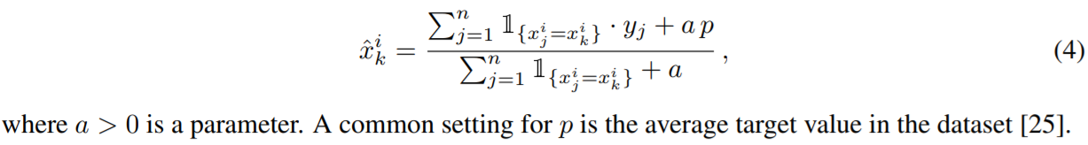
A straightforward approach is to estimate E(y | x  i = x  i  k  ) as the average value of y  over the training examples with the same category x  i  k  [25]. This estimate is noisy for low-frequency  categories, and one usually smoothes it by some prior p:

where a > 0 is a parameter. A common setting for p is the average target value in the dataset [25].  The problem of such greedy approach is target leakage: feature xˆ  i  k  is computed using yk, the target of  xk. This leads to a conditional shift [30]: the distribution of xˆ  i  |y differs for training and test examples.  The following extreme example illustrates how dramatically this may affect the generalization error  of the learned model. Assume i-th feature is categorical, all its values are unique, and for each  category A, we have P(y = 1 | x  i = A) = 0.5 for a classification task. Then, in the training dataset,  xˆ  i  k =  yk+ap  1+a  , so it is sufficient to make only one split with threshold t =  0.5+ap  1+a  to perfectly classify  all training examples. However, for all test examples, the value of the greedy TS is p, and the obtained  model predicts 0 for all of them if p < t and predicts 1 otherwise, thus having accuracy 0.5 in both  cases. To this end, we formulate the following desired property for TS:

一个简单的方法是估计E(y | x i = x i k)作为y除以具有相同类别x i k[25]的训练实例的平均值。对于低频类别，这个估计是有噪声的，人们通常通过一些先验p来平滑它:

其中a> 0是参数。 p的常见设置是数据集中的平均目标值[25]。这种贪婪方法的问题是目标泄漏：特征xˆ i k是使用xk的目标yk计算的。这导致条件转移[30]：对于训练和测试示例，xˆ i | y的分布不同。以下极端示例说明了这可能严重影响学习模型的泛化误差。假设第i个特征是分类的，其所有值都是唯一的，并且对于每个类别A，对于分类任务，我们的P（y = 1 | x i = A）= 0.5。然后，在训练数据集中，xˆ k = yk + ap 1 + a，因此仅对阈值t = 0.5 + ap 1 + a进行一次分割就足以对所有训练示例进行完美分类。但是，对于所有测试示例，贪婪TS的值为p，并且如果p <t，则所获得的模型对所有示例的预测均为0，否则为1，因此在两种情况下的准确度均为0.5。为此，我们为TS制定了以下所需属性：

P1 E(ˆx  i  | y = v) = E(ˆx  i  k  | yk = v), where (xk, yk) is the k-th training example.  In our example above, E(ˆx  i  k  | yk) = yk+ap  1+a  and E(ˆx  i  | y) = p are different.  There are several ways to avoid this conditional shift. Their general idea is to compute the TS for xk  on a subset of examples Dk ⊂ D \ {xk} excluding xk:

P1 E（ˆx i | y = v）= E（ˆi k | yk = v），其中（xk，yk）是第k个训练示例。 在上面的示例中，E（ˆx i k | yk）= yk + ap 1 + a和E（ˆx i | y）= p是不同的。 有几种方法可以避免这种条件转移。 他们的一般想法是在示例xk⊂D \ {xk}的子集中计算xk的TS，不包括xk：

One way is to partition the training dataset into two parts D = Dˆ  0 t Dˆ  1 and use  Dk = Dˆ  0 for calculating the TS according to (5) and Dˆ  1 for training (e.g., applied in [8] for Criteo  dataset). Though such holdout TS satisfies P1, this approach significantly reduces the amount of data  used both for training the model and calculating the TS. So, it violates the following desired property:  

P2 Effective usage of all training data for calculating TS features and for learning a model.

一种方法是训练数据集分割成两部分D = Dˆ0 t Dˆ1和使用Dk = Dˆ0计算TS根据(5)和Dˆ1训练(例如,应用于Criteo数据集[8])。尽管这种Holdout TS满足P1，但这种方法显著减少了用于训练模型和计算TS的数据量。因此，它违反了以下期望的性质:

P2有效使用所有训练数据来计算TS特征和学习模型。

At first glance, a leave-one-out technique might work well: take Dk = D \ xk  for training examples xk and Dk = D for test ones [31]. Surprisingly, it does not prevent target  leakage. Indeed, consider a constant categorical feature: x  i  k = A for all examples. Let n  + be the  number of examples with y = 1, then xˆ  i  k =  n  +−yk+a p  n−1+a  and one can perfectly classify the training  dataset by making a split with threshold t =  n  +−0.5+a p  n−1+a  .

乍一看，留一法技术可能会很好用：对于训练示例xk，使Dk = D \ xk；对于测试样本，使Dk = D [31]。 令人惊讶的是，它不能防止目标泄漏。 实际上，考虑一个恒定的分类特征：对于所有示例，x i k =A。 设n +为y = 1的示例数，则xˆ ik = n + -yk + apn-1 + a，通过对阈值t = n + -0.5 + apn-进行分割，可以完美地对训练数据集进行分类。 1 + a。

CatBoost uses a more effective strategy. It relies on the ordering principle, the  central idea of the paper, and is inspired by online learning algorithms which get training examples  sequentially in time [1, 15, 18, 22]). Clearly, the values of TS for each example rely only on the  observed history. To adapt this idea to standard offline setting, we introduce an artificial “time”, i.e.,  a random permutation σ of the training examples. Then, for each example, we use all the available  “history” to compute its TS, i.e., take Dk = {xj : σ(j) < σ(k)} in Equation (5) for a training  example and Dk = D for a test one. The obtained ordered TS satisfies the requirement P1 and allows  to use all training data for learning the model (P2). Note that, if we use only one random permutation,  then preceding examples have TS with much higher variance than subsequent ones. To this end,  CatBoost uses different permutations for different steps of gradient boosting, see details in Section 5.

CatBoost使用了更有效的策略。它依赖于本文的中心思想——排序原则，并受到在线学习算法的启发，在线学习算法在时间上连续地获取训练示例[1,15,18,22])。显然，每个示例的TS值只依赖于观察到的历史。为了使这一思想适应于标准的离线设置，我们引入了一个人工的“时间”，即训练实例的随机排列σ。然后，对于每个例子，我们使用所有可用的“history”来计算它的TS，即取式(5)中的Dk = {xj:σ(j) <σ(k)}作为训练例，取式(5)中的Dk = D作为测试例。得到的有序TS满足要求P1，允许使用所有训练数据学习模型(P2)。请注意，如果我们只使用一个随机排列，那么前面的例子的TS的方差要比后面的例子大得多。为此，CatBoost对梯度增强的不同步骤使用不同的排列，详见第5节。

In this section, we reveal the problem of prediction shift in gradient boosting, which was neither  recognized nor previously addressed. Like in case of TS, prediction shift is caused by a special kind  of target leakage. Our solution is called ordered boosting and resembles the ordered TS method.  Let us go back to the gradient boosting procedure described in Section 2. In practice, the expectation  in (2) is unknown and is usually approximated using the same dataset D:

在本节中，我们揭示了梯度增强中预测偏移的问题，这个问题既没有被认识到，也没有被解决。与TS情况一样，预测偏移是由一种特殊的目标泄漏引起的。我们的解决方案称为有序助推，类似于有序TS方法。让我们回到第2节中描述的梯度增强过程。在实践中，(2)中的期望是未知的，通常使用相同的数据集D来近似:

Now we describe and analyze the following chain of shifts:  

1. the conditional distribution of the gradient g  t  (xk, yk) | xk (accounting for randomness of  D \ {xk}) is shifted from that distribution on a test example g  t  (x, y) | x;  

2. in turn, base predictor h  t defined by Equation (6) is biased from the solution of Equation (2);  

3. this, finally, affects the generalization ability of the trained model F  t  .  

As in the case of TS, these problems are caused by the target leakage. Indeed, gradients used at each  step are estimated using the target values of the same data points the current model F  t−1 was built on.  However, the conditional distribution F  t−1  (xk) | xk for a training example xk is shifted, in general,  from the distribution F  t−1  (x) | x for a test example x. We call this a prediction shift

现在我们来描述和分析以下的转变链:

1. 将梯度g t (xk, yk) | xk(考虑D \ {xk}的随机性)的条件分布从该分布移到一个检验例g t (x, y) | x上;

2. 反之，由式(6)定义的基预测量h t与式(2)的解有偏倚;

3.这最终影响了训练后的模型F t的泛化能力。

与TS的情况一样，这些问题是由目标泄漏引起的。实际上，每一步使用的梯度都是使用当前模型F t−1所建立的相同数据点的目标值来估计的。然而，训练例xk的条件分布F t−1 (xk) | xk通常从测试例x的分布F t−1 (x) | x移位。我们称之为预测移位

The shift of gradient conditional distribution g  t  (xk, yk) | xk  was previously mentioned in papers on boosting [3, 13] but was not formally defined. Moreover, even  the existence of non-zero shift was not proved theoretically. Based on the out-of-bag estimation [2],  Breiman proposed iterated bagging [3] which constructs a bagged weak learner at each iteration on  the basis of “out-of-bag” residual estimates. However, as we formally show in Appendix E, such  residual estimates are still shifted. Besides, the bagging scheme increases learning time by factor of  the number of data buckets. Subsampling of the dataset at each iteration proposed by Friedman [13]  addresses the problem much more heuristically and also only alleviates it.

梯度条件分布g t (xk, yk) | xk的移位在之前关于Boosting的文献中有提及[3,13]，但没有正式定义。 而且，理论上甚至没有证明非零位移的存在。基于out- bag估计[2]，Breiman提出了迭代bagging[3]，该算法基于out- bag残差估计在每次迭代时构造一个bagging弱学习者。然而，正如我们在附录E中正式说明的那样，这些残差估计仍然发生了偏移。此外，套袋方案通过增加数据桶数量来增加学习时间。Friedman[13]提出的在每次迭代时对数据集进行子抽样的方法更加启发式地解决了这个问题，并且只能缓解该问题。

 We formally analyze the problem of prediction shift in a simple case  of a regression task with the quadratic loss function L(y, yˆ) = (y − yˆ)  2  .  4  In this case, the negative  gradient −g  t  (xk, yk) in Equation (6) can be substituted by the residual function r  t−1  (xk, yk) :=  yk − F  t−1  (xk).  5 Assume we have m = 2 features x  1  , x2  that are i.i.d. Bernoulli random variable with p = 1/2 and y = f  ∗  (x) = c1x  1 + c2x  2  . Assume we make N = 2 steps of gradient boosting  with decision stumps (trees of depth 1) and step size α = 1. We obtain a model F = F  2 = h  1 + h  2  .  W.l.o.g., we assume that h  1  is based on x  1  and h  2  is based on x  2  , what is typical for |c1| > |c2| (here  we set some asymmetry between x  1  and x  2  ).

我们以二次损失函数L（y，yˆ）=（y-yˆ）2的形式简单地分析了回归任务的简单预测转移问题。 4在这种情况下，公式（6）中的负梯度-g t（xk，yk）可以用残差函数r t-1（xk，yk）：= yk-F t-1（xk）代替。 5假设我们有m = 2个特征x 1，x2，即i.d. 伯努利随机变量，其中p = 1/2和y = f ∗（x）= c1x 1 + c2x 2。 假设我们用决策树桩（深度为1的树）且步长为α= 1来进行N = 2步的梯度增强。我们获得模型F = F 2 = h 1 + h 2。 W.l.o.g.，我们假设h 1基于x 1，h 2基于x 2，这对于| c1 | > | c2 | （这里我们在x 1和x 2之间设置了一些不对称性）。

Theorem 1 1. If two independent samples D1 and D2 of size n are used to estimate h  1 and h  2  ,  respectively, using Equation (6), then ED1,D2 F  2  (x) = f  ∗  (x) + O(1/2  n) for any x ∈ {0, 1}  2  .  2. If the same dataset D = D1 = D2 is used in Equation (6) for both h  1 and h  2  , then EDF  2  (x) =  f  ∗  (x) −  1  n−1  c2(x  2 −  1  2  ) + O(1/2  n).  

This theorem means that the trained model is an unbiased estimate of the true dependence y = f  ∗  (x),  when we use independent datasets at each gradient step.6 On the other hand, if we use the same  dataset at each step, we suffer from a bias −  1  n−1  c2(x  2 −  1  2  ), which is inversely proportional to  the data size n. Also, the value of the bias can depend on the relation f  ∗  : in our example, it is  proportional to c2. We track the chain of shifts for the second part of Theorem 1 in a sketch of the  proof below, while the full proof of Theorem 1 is available in Appendix A.  

Sketch of the proof . Denote by ξst, s, t ∈ {0, 1}, the number of examples (xk, yk) ∈ D with  xk = (s, t). We have h  1  (s, t) = c1s +  c2ξs1  ξs0+ξs1  . Its expectation E(h  1  (x)) on a test example x equals  c1x  1 +  c2  2  . At the same time, the expectation E(h  1  (xk)) on a training example xk is different and  equals (c1x  1 +  c2  2  ) − c2(  2x  2−1  n  ) + O(2−n). That is, we experience a prediction shift of h  1  . As a  consequence, the expected value of h  2  (x) is E(h  2  (x)) = c2(x  2 −  1  2  )(1 −  1  n−1  ) + O(2−n) on a test  example x and E(h  1  (x) + h  2  (x)) = f  ∗  (x) −  1  n−1  c2(x  2 −  1  2  ) + O(1/2  n).  

Finally, recall that greedy TS xˆ  i  can be considered as a simple statistical model predicting the target  y and it suffers from a similar problem, conditional shift of xˆ  i  k  | yk, caused by the target leakage, i.e.,  using yk to compute xˆ  i  k  .

定理1 1.如果使用等式（6）分别使用大小为n的两个独立样本D1和D2估计h 1和h 2，则ED1，D2 F 2（x）= f ∗（x）+ O（ 1/2 n）对于任何x∈{0，1} 2。 2.如果对于h 1和h 2在公式（6）中使用相同的数据集D = D1 = D2，则EDF 2（x）= f ∗（x）− 1 n−1 c2（x 2 − 1 2 ）+ O（1/2 n）。

该定理意味着，当我们在每个梯度步骤使用独立的数据集时，训练后的模型是真实依赖关系y = f ∗（x）的无偏估计。6另一方面，如果在每个梯度步骤中使用相同的数据集，我们偏置-1 n-1 c2（x 2-1 2）与数据大小n成反比。同样，偏置值可以取决于关系f ∗：在我们的示例中，它与c2成比例。我们在下面的证明草图中追踪定理1的第二部分的移位链，而定理1的完整证明可在附录A中找到。

证明草图。用ξst，s，t∈{0，1}表示xk =（s，t）的示例数（xk，yk）∈D。我们有h 1（s，t）= c1s +c2ξs1ξs0+ξs1。在测试示例x上的期望E（h 1（x））等于c1x 1 + c2 2。同时，对训练示例xk的期望E（h 1（xk））不同，并且等于（c1x 1 + c2 2）-c2（2x 2−1 n）+ O（2-n）。也就是说，我们经历了h 1的预测偏移。结果，在测试示例中，h 2（x）的期望值是E（h 2（x））= c2（x 2-1 2）（1-1 n-1）+ O（2-n） x和E（h 1（x）+ h 2（x））= f ∗（x）− 1 n-1 c2（x 2 − 1 2）+ O（1/2 n）。

最后，回想一下贪婪的TS xˆ i可以看作是预测目标y的简单统计模型，它也遇到类似的问题，即xˆ i k的条件转移。由目标泄漏引起的yk，即使用yk计算xˆ i k。

Here we propose a boosting algorithm which does not suffer from the prediction shift problem  described in Section 4.1. Assuming access to an unlimited amount of training data, we can easily  construct such an algorithm. At each step of boosting, we sample a new dataset Dt independently  and obtain unshifted residuals by applying the current model to new training examples. In practice,  however, labeled data is limited. Assume that we learn a model with I trees. To make the residual  r  I−1  (xk, yk) unshifted, we need to have F  I−1  trained without the example xk. Since we need  unbiased residuals for all training examples, no examples may be used for training F  I−1  , which at  first glance makes the training process impossible. However, it is possible to maintain a set of models  differing by examples used for their training. Then, for calculating the residual on an example, we use  a model trained without it. In order to construct such a set of models, we can use the ordering principle  previously applied to TS in Section 3.2. To illustrate the idea, assume that we take one random  permutation σ of the training examples and maintain n different supporting models M1, . . . , Mn  such that the model Mi  is learned using only the first i examples in the permutation. At each step, in  order to obtain the residual for j-th sample, we use the model Mj−1 (see Figure 1). The resulting  Algorithm 1 is called ordered boosting below. Unfortunately, this algorithm is not feasible in most  practical tasks due to the need of training n different models, what increase the complexity and  memory requirements by n times. In CatBoost, we implemented a modification of this algorithm on  the basis of the gradient boosting algorithm with decision trees as base predictors (GBDT) described  in Section 5.

这里我们提出了一种提升算法，它不会受到第4.1节中描述的预测偏移问题的影响。假设可以获得无限数量的训练数据，我们可以很容易地构建这样一个算法。在增强的每一步，我们独立地采样一个新的数据集Dt，并通过将当前模型应用到新的训练实例中获得未移位的残差。然而，在实践中，标记数据是有限的。假设我们学习一个有I树的模型。为了使残差r I−1 (xk, yk)不移位，我们需要训练F I−1，而不使用例子xk。由于我们需要对所有的训练例子都有无偏残差，所以不能用任何例子来训练F I−1，乍一看，这使得训练过程不可能进行。然而，由于训练中使用的例子不同，我们可以维护一组不同的模型。然后，为了计算一个实例上的残差，我们使用一个没有残差的训练模型。为了构建这样一组模型，我们可以使用之前在3.2节中应用于TS的排序原则。为了说明这一思想，假设我们取训练实例的一个随机排列σ，并维持n个不同的支持模型M1，…，使模型Mi仅使用排列中的前i个例子来学习。在每一步中，为了得到第j个样本的残差，我们使用模型Mj−1(见图1)，得到的算法1如下所示:ordered boosting。不幸的是，这种算法在大多数实际任务中都不可行，因为需要训练n个不同的模型，这增加了n倍的复杂性和内存需求。在CatBoost中，我们在第5节所述的以决策树作为基础预测器(GBDT)的梯度增强算法的基础上，实现了对该算法的改进。

Ordered boosting with categorical features In Sections 3.2 and 4.2 we proposed to use random  permutations σcat and σboost of training examples for the TS calculation and for ordered boosting,  respectively. Combining them in one algorithm, we should take σcat = σboost to avoid prediction  shift. This guarantees that target yi  is not used for training Mi (neither for the TS calculation, nor for  the gradient estimation). See Appendix F for theoretical guarantees. Empirical results confirming the  importance of having σcat = σboost are presented in Appendix G.

在第3.2节和4.2节中，我们分别提出了使用随机排列σcat和σboost的训练实例进行TS计算和有序增强。将它们结合在一个算法中，我们应该采用σcat =σboost来避免预测偏移。这保证了目标yi不用于训练Mi(既不用于TS计算，也不用于梯度估计)。理论保证见附录F。附录G给出了经验结果，证实了σcat =σboost的重要性。

CatBoost has two boosting modes, Ordered and Plain. The latter mode is the standard GBDT  algorithm with inbuilt ordered TS. The former mode presents an efficient modification of Algorithm 1.  A formal description of the algorithm is included in Appendix B. In this section, we overview the  most important implementation details.

CatBoost有两种模式，有序模式和普通模式。后一种模式是标准的带内置有序TS的GBDT算法，前者是对算法1的有效改进。该算法的正式描述包含在附录b中。在本节中，我们将概述最重要的实现细节。

At the start, CatBoost generates s + 1 independent random permutations of the training dataset. The  permutations σ1, . . . , σs are used for evaluation of splits that define tree structures (i.e., the internal  nodes), while σ0 serves for choosing the leaf values bj of the obtained trees (see Equation (3)). For  examples with short history in a given permutation, both TS and predictions used by ordered boosting  (Mσ(i)−1(xi) in Algorithm 1) have a high variance. Therefore, using only one permutation may  increase the variance of the final model predictions, while several permutations allow us to reduce  this effect in a way we further describe. The advantage of several permutations is confirmed by our  experiments in Section 6.

在开始时，CatBoost对训练数据集生成s + 1个独立的随机排列。排列σ1，…，σs用于评估定义树结构(即内部节点)的分片，而σ0用于选择所获得树的叶值bj(见式(3))。例如，在给定的排列中历史很短，有序提升使用的TS和预测(算法1中的Mσ(i)−1(xi))都有很大的方差。因此，仅使用一种排列可能会增加最终模型预测的方差，而使用几种排列则允许我们以进一步描述的方式减少这种影响。我们在第6节的实验证实了几种排列的优点。

Building a tree In CatBoost, base predictors are oblivious decision trees [9, 14] also called decision  tables [23]. Term oblivious means that the same splitting criterion is used across an entire level of the  tree. Such trees are balanced, less prone to overfitting, and allow speeding up execution at testing  time significantly. The procedure of building a tree in CatBoost is described in Algorithm 2.  

In the Ordered boosting mode, during the learning process, we maintain the supporting models Mr,j ,  where Mr,j (i) is the current prediction for the i-th example based on the first j examples in the  permutation σr. At each iteration t of the algorithm, we sample a random permutation σr from  {σ1, . . . , σs} and construct a tree Tt on the basis of it. First, for categorical features, all TS are  computed according to this permutation. Second, the permutation affects the tree learning procedure.

Namely, based on Mr,j (i), we compute the corresponding gradients gradr,j (i) = ∂L(yi,s)  ∂s      s=Mr,j (i)  .  Then, while constructing a tree, we approximate the gradient G in terms of the cosine similarity  cos(·, ·), where, for each example i, we take the gradient gradr,σ(i)−1(i) (it is based only on the  previous examples in σr). At the candidate splits evaluation step, the leaf value ∆(i) for example i is  obtained individually by averaging the gradients gradr,σr(i)−1 of the preceding examples p lying  in the same leaf leafr(i) the example i belongs to. Note that leafr(i) depends on the chosen  permutation σr, because σr can influence the values of ordered TS for example i. When the tree  structure Tt (i.e., the sequence of splitting attributes) is built, we use it to boost all the models Mr  0  ,j .  Let us stress that one common tree structure Tt is used for all the models, but this tree is added to  different Mr  0  ,j with different sets of leaf values depending on r  0  and j, as described in Algorithm 2.  

The Plain boosting mode works similarly to a standard GBDT procedure, but, if categorical features  are present, it maintains s supporting models Mr corresponding to TS based on σ1, . . . , σs.

在CatBoost中，基本的预测器是oblivious决策树[9,14]，也称为决策表[23]。术语无关是指在整个树的层次上使用相同的分割标准。这样的树是平衡的，不容易过度拟合，并允许在测试时间显著加快执行。在CatBoost中建立树的过程在算法2中描述。

在有序提升模式中，在学习过程中，我们保持支持模型Mr,j，其中Mr,j (i)是基于排列σr中前j个例子的对第i个例子的当前预测。在算法的每一次迭代t中，我们从{σ1，…，σs}，并在此基础上构造树Tt。首先，对于类别特征，根据这种排列计算所有的t。其次，排列影响树的学习过程。

即，基于Mr,j (i)，计算相应的梯度gradr,j (i) =∂L(yi,s)∂s s=Mr,j (i)。然后，在构造树的时候，我们用余弦相似度cos(·，·)来近似梯度G，其中，对于每个例子i，我们取梯度梯度r，σ(i)−1(i)(它仅基于之前的σr例子)。在候选拆分评估步骤中，叶片值∆(i)例如i分别通过对位于示例i所属叶片r(i)中的上述示例p的梯度gradr、σr(i)−1进行平均得到。注意，leafr(i)依赖于所选择的排列σr，因为σr可以影响有序TS的值，例如i。让我们强调一下，所有的模型都使用了一种常见的树结构Tt，但是这棵树根据r0和j的不同，被添加到不同的Mr 0,j上，有不同的叶片值集，如算法2所述。

纯提升模式的工作原理与标准的GBDT过程相似，但是，如果有分类特征，它在σ1的基础上保持与TS对应的s支持模型Mr，…σs。

Choosing leaf values Given all the trees constructed, the leaf values of the final model F are  calculated by the standard gradient boosting procedure equally for both modes. Training examples i  are matched to leaves leaf0(i), i.e., we use permutation σ0 to calculate TS here. When the final  model F is applied to a new example at testing time, we use TS calculated on the whole training data  according to Section 3.2.

在给定所有构建的树的情况下，最终模型F的叶子值在两种模式下均通过标准梯度增强程序计算。训练示例i与叶子leaf0(i)匹配，即我们在这里使用排列σ0来计算TS。当在测试时将最终的模型F应用到一个新的示例时，我们使用3.2节对整个训练数据计算的TS。

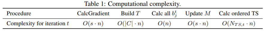
Complexity In our practical implementation, we use one important trick, which significantly  reduces the computational complexity of the algorithm. Namely, in the Ordered mode, instead  of O(s n2  ) values Mr,j (i), we store and update only the values M0  r,j (i) := Mr,2  j (i) for j =  1, . . . , dlog2 ne and all i with σr(i) ≤ 2  j+1, what reduces the number of maintained supporting  predictions to O(s n). See Appendix B for the pseudocode of this modification of Algorithm 2.  

In Table 1, we present the computational complexity of different components of both CatBoost modes  per one iteration (see Appendix C.1 for the proof). Here NT S,t is the number of TS to be calculated at  the iteration t and C is the set of candidate splits to be considered at the given i